How to Format - Font.

Microsoft Excel lets you change many of the ways it displays data in a cell. For example, you can specify the number of digits to the right of a decimal point, or you can add a pattern and border to the cell or you can adjust your fonts to something easier on the eye.

FONT

A font is a specific typeface of a certain size and style. For example, one font may be Arial 12 pt bold, while another font may be Times New Roman 14 pt italic. Most word processing programs have a Font menu that allows you to choose the typeface, size, and style of the text.

Change the font type of text in a cell(s) by clicking on the drop down in the Home tab of the Ribbon.

Since your text will appear in small cells (generally speaking), we think that it is especially important to choose a clear font. It is recommend that sans serif fonts are used, such as:

 Calibri size, 11 (2007 default)

 Arial, size 10 (2003 default)

 Franklin Gothic Book, size 11

Font size

Font size can also be changed with the drop-down on the Home tab of the Ribbon. Of course it depends which font face you’ve chosen and how you like to view the sheet, but in general using and sticking to font size 10, 11 or 12 works well.

Increasing / decreasing font size

These two buttons:

will increase or decrease the font size respectively.

Typeface Styles:  Bold, italic, underline

The three adjacent buttons:

Embolden, italicise and underline (with shortcuts Ctrl-B, Ctrl-I and Ctrl-U) respectively.

The list of choices in the Font Style list varies depending on the font that is selected in the Font list. Most fonts include the following styles:

·  Regular

·  Italic

·  Bold

·  Bold italic

Underline

In the Underline list, you can select an underlining option to format the selected text. The following table describes each underlining option:

   Underline type        Description

   -----------------------------------------------------------------------

   None                  No underlining is applied.

   Single                A single underline is placed under each character

                         in the cell. The underline is drawn through the

                         descenders of characters like "g" and "p."

   Double                Double underlines are placed under each character

                         in the cell. The underlines are drawn through the

                         descenders of characters like "g" and "p."

   Single Accounting     A single underline is placed across the entire

                         width of the cell. The underline is drawn below

                         the descenders of characters like "g" and "p."

   Double Accounting     Double underlines are placed across the entire

                         width of the cell. The underlines are drawn below

                         the descenders of characters like "g" and "p."

Font colour

Last of the controls on the Font group is the Font Colour icon.

Used the same way as the others, it changes the colour of your text. In the interests of simplicity and clarity we recommend using black, the default (aka ‘Automatic’), unless you have very good reason for doing otherwise. One good exception to this is the practice of using red text for negative numbers.

Next time we’ll cover cell Borders and Shading............

Simply Navigating

Navigating:-

Moving around the spreadsheet. With the vast size of so many spread sheets, one needs to learn how navigate to and find the information that one is looking for.

The simplest way would be by using the mouse to click on the section on the spreadsheet required, or to use the pointer to select your desired direction on the scroll bars. When using the mouse: left clicking on a cell selects that cell; holding down the left mouse button and moving the pointer selects a rectangle of cells.

Some other options are:

·  Arrow keys. These move the selected cell one cell at a time in the arrow’s direction. 

·  The 'Enter Key'. Has the same effect as the down arrow (¯) – moves a cell down

·  Page up/down. This scrolls up/down by a ‘page’ – that is, by the height of the spreadsheet that is visible in the window. The selected cell will move a page up or down too.

·  Ctrl key plus arrow key. This moves the selected cell to the edge of the block of data the selection is on, or if it is not on a block of data to the start of the next one, or, if there are no more blocks of data, to the edge of the spreadsheet.

The Ctrl ® moves the selected cell to the right hand edge of the first block of text; pressing Ctrl ® again jumps to the start of the next block of text, and so on. This is useful in particular if you are working with databases that include blocks of text that are bigger than a single screen.

Holding down Shift while doing any of the navigation tips in the previous section selects all the cells between the start and end point of the selection. So for instance, Shift-Ctrl-¯ with a cell selected, selects all the cells in column below that cell up to the edge of the data block.

The Ribbon and what it does:-

In computing, a ribbon is a set of toolbars placed on several tabs. Graphical buttons and other controls, are grouped by functionality. Such ribbons use tabs to expose different sets of controls, eliminating the need for many parallel toolbars. Contextual tabs are tabs that appear only when the user needs them. For instance, in a word processor, an image-related tab may appear when the user selects an image in a document, allowing the user to interact with that image.

Tools and the ribbon:-

‘Find & Select’ searches the spreadsheet for a word or other set of characters. If those characters exist in a cell, Find will select that cell. The Find icon is found on the right of the Home tab of the Ribbon. Click this and then select Find… from the resultant menu.

This results in a box requesting the search text. In that box, you type the word that your are searching for.

Pressing the Find Next button further times finds any further examples of the characters / words / numbers in the spreadsheet.

The Options >> button in the screenshot above enables searching for the text only where it matches all the text in the cell. So for example, if the cell in the above example contained the text ‘Jupiter – planet’, that cell would not have been selected by the search:

A simple start.

As we start the new year. I begin a new challenge in publishing my first blog. I have become a bigger and bigger fan of the spreadsheet (Microsoft Excel in particular) over my working years. Every day I learn something new that can assist me in making my job easier, simpler, more efficient and of course more interesting. I love sharing my new knowledge and skills with whomever will listen and show some interest in the same topics.

As the title of this article states, 'A simple start', this is precisely what I achieve to aim and provide a 'friendly' channel for the Excel novice. This blog has a back to basics agenda which will turn more in depth as our skills develop.

In order to get the most out of the program you will need to become very familiar with the interface. There are few differences between 2007 and 2010.

1. A Simple Start. You ask: "What is Excel?"

Excel is a tool that helps us to understand data better by laying it out in ‘cells’, which combine to form rows and columns.  The diagram below shows what an Excel sheet looks like:-
- The rectangles are cells.
- Each cell has a name according to its location. The name is defined by the   letter at the top of the column (column run vertically - top to bottom) and the number of the row (rows run horizontally - left to right).
- The cell is named at the point where the column and row intersect (meet) - e.g Top left cell would be called A1, the one to the right would be called B1 and the one below A1 would be called A2.

We enter information into each cell and lay it out into a table with column headings and row headings.

In the spreadsheet itself you will only see 30 or so rows and 20 or so columns when you open a new workbook, there are in fact over 1,000,000 rows and over 16,000 columns in Excel 2007. This vast sheet can accommodate a huge amount of data and calculations.
Just click on any cell to start typing numbers or text into it. Then move around the spreadsheet with the arrow keys or by clicking on cells with your mouse pointer.

If you want to highlight the whole of column B you can click on the letter B itself:

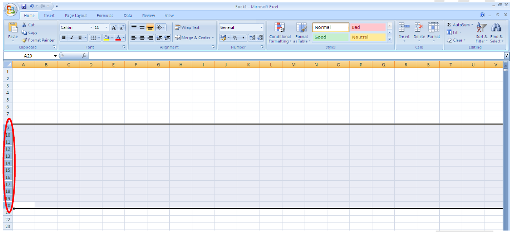
Similarly for a row or collection of rows (for more than one row click on a number to the left, hold the mouse and drag up or down):  

Lastly, you can even click on the top left square to highlight the entire sheet:  

This might be useful to clear all the data or format everything the same way.

My next blog will discuss the task bars, scroll bars and how to navigate in Excel.